This is a follow up to my previous post about Finite Plinko. If you did not read it yet, you can find it here.
Finite Plinko is fun and all but what if we went further? The challenge problem listed at the bottom of the homework assignment asked at what height, if any, the distribution of the expected final location of the dropped disc would become uniform. Solving this as a combination of increasingly longer bounded random variables was too difficult to do properly. However, what we can do instead is treat it like a Markov chain. (Editor’s note: This is not intended to serve as a perfect explanation of what a Markov chain is. It simply is intended to walk us through applying them to the Plinko problem.)
A Markov chain is a stochastic model that represents a possible series of events where the probability of the next event is only dependent on the result of the previous. Now that sounds really fancy and convoluted but what does that really mean?
Imagine you are sleepwalking. Luckily for you, the doors connecting the rooms in your house are mostly closed. You can only get to your bedroom (B), living room (L), and your kitchen (k). When you are sleepwalking, you randomly move along one of your available paths with varying probabilities. We can represent this problem with the following chain:

Here you can see all of the potential paths that you can take from any given room and the likelihood that you take that path. From this, we can compute the likelihood that you are in any given room after any number of random walks. We do this by creating a transition matrix.
A transition matrix is a matrix that represents the likelihood that you move from any node to any other after a single random walk. For this chain, we can create the following matrix:

The row serves as the “input” to the system. So the probability that you move from the kitchen to the living room can be seen to be .25. Notice that each row sums to exactly 1. This means that this matrix is a valid stochastic matrix. That’s a fancy way of saying that it represents valid probabilities. This matrix allows us to calculate the probability of an end location from any start location after an arbitrary number of random walks.
But what does that even mean? Well, we can apply it for just one walk. You start sleepwalking from your bedroom. That means that after one random walk, there is a probability of .5 that you end in your living room and a probability of .5 that you end up in your kitchen. We can even use matrix multiplication to get these end locations. Say you want to determine the likelihood that you end in any location if you start in your kitchen. We can calculate this by simply multiplying this transition matrix by a vector. The vector has the value 1 in the location that corresponds to the starting room and has the value 0 for all other locations.

In this instance, the resulting vector is simply the bottom row of the transition matrix. We can now use this technique to determine the probability of ending in any location after any number of moves. This can be done in one of two ways. You could take this resulting vector and multiply it by the transition matrix to get a new resulting vector. You can continue to do this however many times you would like until you have found your desired answer. Unfortunately, if you want to determine the ution for your end locations after n walks, you have to repeat this step n times. Alternatively, we can just raise the transition matrix to the power n prior to multiplying it by the initial vector. This provides the same result and requires far less steps.
Let’s calculate the likelihood that you end in the living room after taking two random walks from the kitchen. To do this, we can just repeat the last multiplication but use the square of the transition matrix instead.

Using this resulting vecotr, we can see that the probability that we are in the living room after taking two random walks from the kitchen is .4375.
This is cool on its own but now we can apply this knowledge to solve for the real game of Plinko. At first, I’m going to cover a much smaller Plinko board to explain the general idea then move away from these nice images to good ol’ Python.
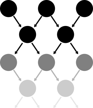
Picture a small, rectangular Plinko board with height 2. The board has 3 pegs in its wide row and 2 pegs in its thin row. The disc encounters one of the top pegs, one of the inner pegs, then falls into a bucket. We can draw arrows to represent all possible paths that a disc can take.

If you take a look at the top row, you can see that the outermost pegs only allow the disc to move in one direction. This is because there is an unmarked boundary wall at these two locations. You can now think of this like a markov chain. Instead of having those buckets be mere buckets, you can picture them as nodes that lead nowhere.

Now that we have a Markov chain that represents the smallest possible sub-problem, we can combine many instances of this problem into a larger one. Imagine that instead of those bottom nodes being buckets, they instead were the top of another set of two rows.
With this image, we can imagine the plinko board continuing on indefinitely. Luckily, using Markov chains, we can solve for this individual sub-problem. First we need to change the way that we think of the problem.
Currently, every top row is considered to be the start of a new sub-problem. But since every new sub-problem is the same as the last, we don’t need to have an infinite number of rows to represent an infinite length board. We can instead think of the chain as returning to the top instead of continuing through the bottom.

This works well but there is another problem that we must solve. The purpose of creating this chain is so we can use it to easily find the probability that it ends in any given bucket. However, we consider the disc to have landed in the bucket if and only if it has just fallen from a thin row of pegs. This means that we can only check for the resulting distribution every other random walk. This periodicity of our ability to sample simply will not do. We instead need to collapse the idea of a walk between 2 rows to a single walk between 3 nodes.
We can get the probability that it returns to its initial location by simply multiplying the probability for each walk. So the probability that the disc begins at the left peg and returns to the left peg is the probability that it moves to the right times the probability that the disc then moves to the left: . We can use this method to determine the edge probabilities for all random walks.

Using this chain, we can now solve for the stationary distribution of our simple rectangular Plinko board. The stationary distribution gives us the likelihood that the random walk ends at any one of the nodes as the number of walks approaches infinity. We do this by calculating the eigenvectors of the matrix. We then select the eigenvector that corresponds to the largest eigenvalue. Since this is a stochastic row matrix, the leading eigenvalue will be 1.
In order to avoid having to actually do this math myself, I’m going to instead input the matrix in Python and have NumPy do the work for me. Most of this Python code comes from Dan Larremore because his was far cleaner than what I had done.
import numpy as np

M = np.zeros([3,3])
p = .5
for i in range(1,2):
    M[i,i] = 2*p*(1-p)
    M[i,i+1] = p**2
    M[i,i-1] = (1-p)**2
M[0,0] = 1-p
M[0,1] = p
M[-1,-1] = p
M[-1,-2] = 1-p
print(M, '\n')

w,v = np.linalg.eig(np.transpose(M))

steadystate = v[:,w==np.max(w)]

steadystate = steadystate/steadystate.sum()
print(steadystate)
[[ 0.5   0.5   0.  ]
 [ 0.25  0.5   0.25]
 [ 0.    0.5   0.5 ]]

[[ 0.25]
 [ 0.5 ]
 [ 0.25]]
This gives us the transition matrix of the simple game of Plinko followed by the standing distribution. We can interpret this as saying that as the number of random walks approaches infinity, the probability of being at the center peg approaches .5.
With this standing distribution, we have solved infinite Plinko… for this smaller board. Now all we have to do is scale this up to meet the requirements for the full-sized board. Instead of having rows with a width of 3 and 2, the full board has rows of sizes 9 and 8. With a simple change to this code, we can have it calculate the standing distribution of this larger board:
T = np.zeros([9,9])
for i in range(1,8):
    T[i,i] = 2*r*(1-p)
    T[i,i+1] = p**2
    T[i,i-1] = (1-p)**2
T[0,0] = 1-p
T[0,1] = p
T[-1,-1] = p
T[-1,-2] = 1-p
print(T, '\n')

w,v = np.linalg.eig(np.transpose(T))

steadystate = v[:,w==np.max(w)]

steadystate = steadystate/steadystate.sum()
print(steadystate)
[[ 0.5   0.5   0.    0.    0.    0.    0.    0.    0.  ]
 [ 0.25  0.5   0.25  0.    0.    0.    0.    0.    0.  ]
 [ 0.    0.25  0.5   0.25  0.    0.    0.    0.    0.  ]
 [ 0.    0.    0.25  0.5   0.25  0.    0.    0.    0.  ]
 [ 0.    0.    0.    0.25  0.5   0.25  0.    0.    0.  ]
 [ 0.    0.    0.    0.    0.25  0.5   0.25  0.    0.  ]
 [ 0.    0.    0.    0.    0.    0.25  0.5   0.25  0.  ]
 [ 0.    0.    0.    0.    0.    0.    0.25  0.5   0.25]
 [ 0.    0.    0.    0.    0.    0.    0.    0.5   0.5 ]]

[[ 0.0625]
 [ 0.125 ]
 [ 0.125 ]
 [ 0.125 ]
 [ 0.125 ]
 [ 0.125 ]
 [ 0.125 ]
 [ 0.125 ]
 [ 0.0625]]
There we have it. The stationary distribution of the full-size Plinko board is not uniform. Therefore, there is no height at which the probability of landing in each bucket is identical.
Note: It would be remiss of me to not clarify one aspect of this problem. While I found the stationary distribution to not be uniform, Dan initially found it to be uniform. We realized that the discrepancy arose because of the way that we defined the problem itself. In my setup, the chain defines the movement from the larger row to the shorter row then back to the larger row. However, Dan structured the problem going from the short row to the large row as the first random walk. Though these are technically both valid interpretations of the problem, I’d argue that the solution that is more true to the real board is what I have discussed here today. The real Plinko board has the same number of buckets as there are pegs in its wider rows.
With that out of the way, we can start to see a pattern in these stationary distributions. The outer buckets have a probability that is exactly the other buckets. In fact, we can create a general form of the stationary distribution where is the width of the wider rows and :
Each of these fractions corresponds to a different bucket at the bottom of the infinite length board. This means that there is no width such that the distribution is uniform.
This concludes our exploration into the wonderful world of Plinko. Solving infinite forms of seemingly simple problems is surprisingly interesting. Maybe I’ll find another to do.